Why My PostgreSQL Slow Right After Insert

The Customer Claim That Exposed PostgreSQL’s Statistics Blind Spot

It started with a client claim: a critical part of their workflow was unresponsive. Upon investigation, we found the bottleneck was an innocent-looking query that was now consistently timing out. To understand why, we had to descend into the internals of the PostgreSQL query planner. There, we discovered a rare bug in statistics estimation triggered by a unique data distribution pattern that had remained hidden until now.

This post documents that journey. It’s long because the bug is subtle, and understanding why it happens requires walking through how PostgreSQL’s optimizer makes decisions. If you’ve ever seen a query plan go sideways for no apparent reason, or wondered why PostgreSQL sometimes chooses a nested loop when a hash join seems obvious, this might be relevant to your work.

Thanks for sticking with the technical details. The payoff is understanding a class of performance problems that won’t show up in most tutorials or documentation.

My Join Query Was Slow… But Only Sometimes

The bug report came in like most production mysteries do: a feature that had worked flawlessly for years suddenly started timing out. What made it particularly frustrating was that it only happened in one specific production environment out of dozens running the same code.

The architecture was straightforward. Our system processes jobs by distributing work across multiple workers. During execution, each worker saves individual results to PostgreSQL. After all workers complete, an aggregation step runs a join query to compute final statistics across the results.

When we checked Elastic APM and the logs, we found something odd: the aggregation query would take 60+ seconds immediately after the bulk insert completed, causing timeouts. But when we manually re-ran the exact same query minutes later, it completed in under a second.

The query itself was a standard 4-table join following this structure:

A <-> B <-> C <-> D

Table A contained 1 row, B had around 1,000 rows, C ranged from 100 to 1,000 rows, and D had 1-10 rows. Due to the join relationships, the intermediate result set could balloon to millions of rows before aggregation.

On paper, this should be fine. PostgreSQL’s Hash Join is designed to handle exactly this kind of scale efficiently. We had proper indexes on all foreign keys. The same query processed similar data volumes without issues in other environments.

Yet here we were, with a query that was inexplicably slow right after data creation, then mysteriously fast minutes later—only in this one environment.

What Does the Query Planner Say?

I ran EXPLAIN (ANALYZE, BUFFERS) on both fast and slow executions:

-- The query structure
SELECT *
FROM table_a a
JOIN table_b b ON a.id = b.a_id
JOIN table_c c ON b.id = c.b_id
JOIN table_d d ON c.id = d.c_id
WHERE a.job_id = $1;

The key differences between the plans:

Fast execution:

• Nested Loop joins throughout
• Row estimates closely matched actuals (within 10-20%)
• Total cost estimate: ~15,000

Slow execution:

• Hash Join chosen for the C→D join
• Row estimate at C→D join: 500 rows
• Actual rows at C→D join: 45,000 rows
• Hash table exceeded work_mem, causing disk spills
• Total cost estimate: ~12,000 (lower than the fast plan!)

The planner estimated the Hash Join would be cheaper, but the massive underestimate of row counts at the third join caused it to build an oversized hash table that spilled to disk. Each disk spill added seconds of I/O overhead.

The smoking gun: pg_stat_user_tables showed table_c hadn’t been analyzed in 8 days, during which the related data for this particular job_id had grown significantly. The planner was making decisions based on stale statistics.

Running ANALYZE on all four tables immediately stabilized the query—subsequent executions consistently chose Nested Loop joins and completed in under 200ms.

The Culprit: Nested Loop Instead of Hash Join

EXPLAIN ANALYZE showed PostgreSQL switching join algorithms. Most of the time it chose a hash join. Right after bulk inserts, it switched to a nested loop join.

Nested loop joins scan one table repeatedly for each row in the other table. With large datasets and no selective indexes on the join columns, this becomes a performance killer. Hash joins build a hash table once and probe it, making them dramatically faster for this pattern.

PostgreSQL chooses nested loops when it estimates one side of the join returns few rows. After bulk inserts, stale statistics made it guess wrong.

Join Algorithms Refresher

Database systems have three main join algorithms, each with distinct performance characteristics. Choosing the wrong one can mean the difference between a query that completes in milliseconds versus one that runs for hours.

Nested Loop Join

The nested loop join is the most straightforward algorithm. For each row in the outer table (the driving table), it scans through every row in the inner table, testing the join condition.

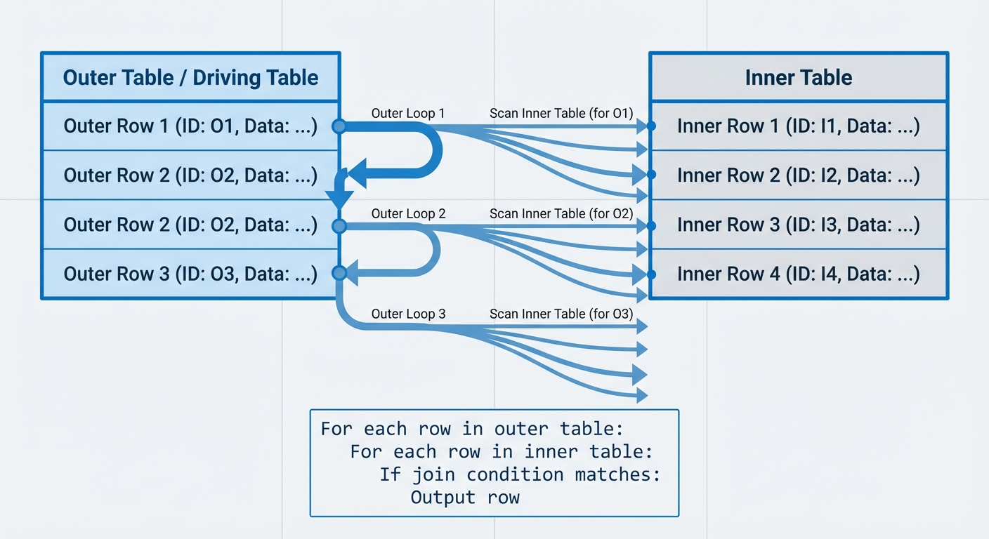
Complexity: O(n*m) where n is rows in the outer table and m is rows in the inner table.

For each row in outer table:
    For each row in inner table:
        If join condition matches:
            Output row

Driving table selection matters, but not for the reasons you might think. Whether you scan 100 rows against 10,000 or 10,000 rows against 100, you’re still making 1,000,000 comparisons. The real benefit appears when the inner table has an index: you get 100 × O(log 10,000) ≈ 1,300 operations versus 10,000 × O(log 100) ≈ 66,000 operations. Without indexes, driving table selection mainly affects cache locality and how effectively you can push down filter conditions on the outer table.

Index Nested Loop Join

In practice, databases rarely use the naive nested loop described above. When an index exists on the inner table’s join key, the algorithm becomes an index nested loop join:

For each row in outer table:
    Use index to find matching rows in inner table (O(log m))
    Output matches

Complexity: O(n × log m) with a B-tree index on the inner table.

This variant is extremely common in production queries. It’s why you’ll often see nested loop joins perform well even with moderately large tables—the index eliminates the full inner table scan.

When nested loop works:

• Small outer table with indexed inner table
• When only a few rows from the outer table match a filter condition
• Small datasets where total comparisons remain manageable

When it fails: Large table joins without indexes on the inner join key. A 1 million × 1 million unindexed join means 1 trillion comparisons.

Hash Join

Hash join builds a hash table from the smaller input table, then probes it with rows from the larger table.

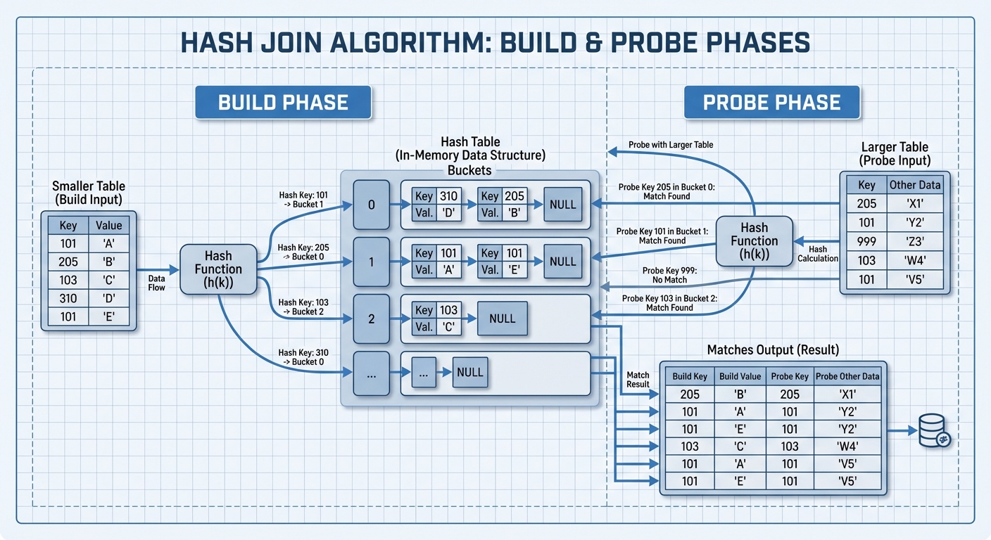
Complexity: O(n+m) - linear in the total number of rows.

Build phase:

1. Scan the smaller table
2. Hash each row’s join key
3. Store the row in a hash table bucket

Probe phase:

1. Scan the larger table
2. Hash each row’s join key
3. Look up matching rows in the hash table
4. Output matches

Memory and hybrid hash join

PostgreSQL uses the work_mem parameter to control hash table size. When the hash table fits in memory, hash join is extremely fast. When the build input exceeds work_mem, PostgreSQL switches to hybrid hash join with batching:

1. Partition both input tables into batches using a hash function
2. Process each batch pair sequentially
3. Each batch’s hash table fits in work_mem

This batching approach maintains predictable performance even with limited memory, though it requires multiple passes over the data (one per batch) and temporary disk space.

When hash join works:

• Large equi-joins (joins using equality like table_a.id = table_b.id)
• When sufficient memory is available for the hash table
• No indexes exist on join keys

Limitations:

• Only works for equi-joins (can’t do <, >, or other non-equality conditions)
• Requires enough work_mem or disk space for batching
• Build phase must complete before any results are returned

Merge Sort Join

Merge sort join requires both inputs to be sorted on the join key, then merges them in a single pass, similar to the merge step in merge sort.

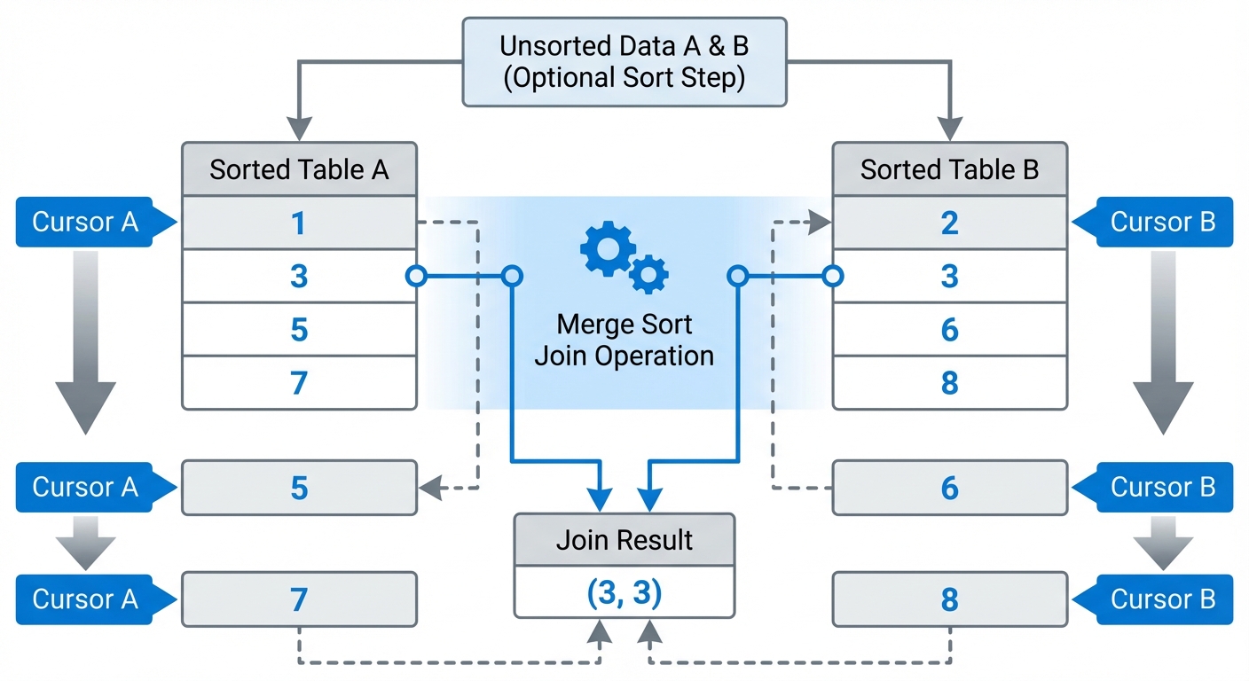
Complexity: O(n log n + m log m) for sorting both inputs (using comparison-based sorting), plus O(n+m) for the merge phase.

If the data is already sorted (due to an index or previous operation), the sort cost disappears and you’re left with just O(n+m).

Algorithm:

1. Sort both tables by join key (if not already sorted)
2. Maintain a pointer in each sorted table
3. Compare current rows
4. If match, output and advance both pointers
5. If no match, advance the pointer with the smaller value

Handling duplicates

When multiple rows share the same join key (many-to-many joins), the algorithm must produce the cartesian product of matching rows. This requires mark/restore operations: the algorithm marks a position in one input, scans through all matches in the other input, then restores the mark position to handle the next matching row. For large groups of duplicates, this may require buffering rows in memory.

When merge join works:

• Data is already sorted or has a usable sort order from indexes
• The query result needs to be ordered anyway (cost is amortized)
• Join condition uses inequality operators (<, >, <=, >=)
• Very large tables where hash join would exceed memory

Trade-offs: The sorting cost can be expensive if data isn’t pre-sorted. However, if you need sorted output for an ORDER BY clause, that cost gets amortized across the query.

Now that we understand why algorithm choice matters, the next question is how PostgreSQL decides which algorithm to use.

Into The Madness: PostgreSQL Query Planner

Before PostgreSQL executes your query, it evaluates multiple execution strategies and estimates the cost of each. The query planner’s job is to pick the lowest-cost path—whether that’s a sequential scan, index scan, nested loop join, or hash join.

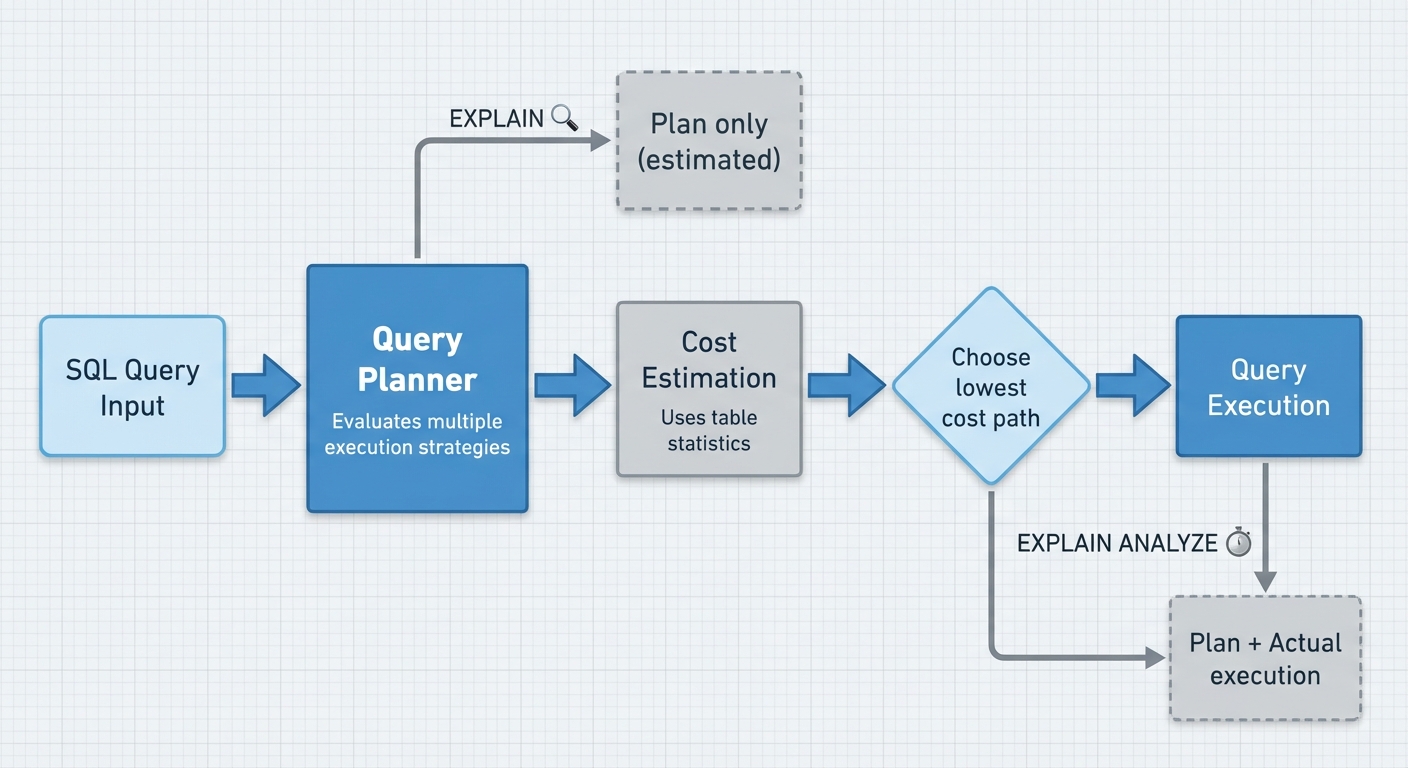
EXPLAIN vs EXPLAIN ANALYZE

EXPLAIN shows the planner’s execution plan without running the query—estimated costs, row counts, and strategies based on table statistics.

EXPLAIN ANALYZE executes the query and shows both the plan and real execution metrics. Use this for SELECT queries to compare estimates against reality. Be careful with DML operations (INSERT/UPDATE/DELETE)—ANALYZE will execute them unless you wrap the statement in a transaction and roll back.

EXPLAIN (ANALYZE, BUFFERS, FORMAT TEXT)
SELECT * FROM table_a a
JOIN table_b b ON a.id = b.a_id
WHERE a.job_id = 123;

Key Options

ANALYZE: Execute the query and show actual timing and row counts. Without this, you only get estimates.

BUFFERS: Show buffer usage—how many blocks were read from shared buffers (cache), how many required disk I/O. This is critical for identifying I/O bottlenecks.

FORMAT: TEXT (default, human-readable), JSON, XML, or YAML. Use JSON when parsing programmatically; stick with TEXT for manual analysis.

VERBOSE: Shows additional details like output column lists and table aliases. Useful when debugging aliasing or column pruning issues.

TIMING: Enabled by default with ANALYZE. Measures actual execution time for each node. You can disable it (TIMING FALSE) on queries with millions of row iterations where timing overhead becomes significant.

Reading Execution Plans

Each line in an execution plan is a node representing an operation. Nodes are indented to show parent-child relationships—inner nodes execute before outer ones.

Nested Loop  (cost=0.56..123.45 rows=10 width=64) (actual time=0.032..0.089 rows=8 loops=1)
  ->  Index Scan using table_a_job_id_idx on table_a a  (cost=0.28..8.30 rows=10 width=32) (actual time=0.015..0.021 rows=8 loops=1)
        Index Cond: (job_id = 123)
        Buffers: shared hit=3
  ->  Index Scan using table_b_pkey on table_b b  (cost=0.28..11.50 rows=1 width=32) (actual time=0.006..0.006 rows=1 loops=8)
        Index Cond: (a_id = a.id)
        Buffers: shared hit=16

Cost: The first number (0.56) is startup cost—work before the first row can be returned. The second number (123.45) is total cost assuming all rows are retrieved. Cost is cumulative—a node’s total cost includes all child node costs. Cost units are based on seq_page_cost, random_page_cost, and cpu_tuple_cost configuration settings. Compare plans relative to each other, not as absolute values.

Rows: Estimated number of rows the planner expects this node to return. Compare this with the actual row count.

Width: Estimated average row size in bytes.

Actual time: Real execution time in milliseconds. First number is time to first row, second is total time. Both are per loop.

Rows (actual): How many rows were actually returned. If this wildly differs from the estimate, the planner might be using stale statistics.

Loops: How many times this node executed. Critical: multiply actual time by loops to get total elapsed time for that node. An index scan taking 0.1ms over 100,000 loops = 10,000ms = 10 seconds of execution time.

Buffers: Each buffer is 8KB. Shows shared hit (blocks read from cache), shared read (disk I/O), shared dirtied (blocks modified), and temp read/temp written (when work_mem is exceeded). shared hit=3 means 24KB read from cache. High shared read indicates disk I/O bottlenecks; temp operations indicate work_mem exhaustion.

Parallel Plans

Modern PostgreSQL uses parallel execution for expensive queries. Look for Parallel Seq Scan or Gather nodes. If Workers Planned exceeds Workers Launched, PostgreSQL couldn’t allocate enough background workers—check max_parallel_workers_per_gather (per-query limit) and max_parallel_workers (system-wide limit), plus current system load.

What To Look For

• Estimate mismatches: When estimated rows differ from actual rows by 10x or more, the planner made bad decisions. A 2-3x mismatch is often acceptable, but 10x+ indicates statistics problems or complex predicates the planner can’t model accurately.
• Sequential scans on large tables: Often fine for small tables or when fetching most rows, but a red flag if you expected an index scan.
• Nested loops with high loop counts: Each iteration runs the inner query again. If the inner side is expensive and loops run 10,000 times, you’re in trouble.
• High buffer reads: If shared read dominates, you’re hitting disk. Consider adding indexes or increasing shared_buffers.

Table Statistics: The Foundation of Query Planning

The query planner estimates costs using statistics from pg_stats, collected by the ANALYZE command. All cardinality estimates derive from these statistics.

-- View statistics for a specific table and column
SELECT
  schemaname,
  tablename,
  attname,
  null_frac,
  n_distinct,
  most_common_vals,
  most_common_freqs,
  histogram_bounds,
  correlation
FROM pg_stats
WHERE tablename = 'your_table'
  AND attname = 'your_column';

Run ANALYZE table_name to update these statistics. Autovacuum handles this automatically, but manual ANALYZE may be necessary after bulk data changes or significant updates.

Key Statistics Explained

null_frac: Fraction of NULL values in the column (0.0 to 1.0). A value of 0.15 means 15% of rows are NULL. Directly affects selectivity for IS NULL and IS NOT NULL predicates.

n_distinct: Estimated number of distinct values. Positive values are absolute counts; negative values are fractions of total rows. For n_distinct = -0.5 with 10,000 rows, the estimate is abs(-0.5) * 10000 = 5,000 distinct values. Critical for estimating join cardinalities and GROUP BY operations.

most_common_vals: Array of most frequent values in the column. The default_statistics_target setting (default: 100) influences how many MCVs are collected, but the actual number stored depends on data distribution—columns with highly skewed data may have many MCVs, while uniform distributions may have few or none. The planner uses exact frequencies for these values rather than statistical estimates.

most_common_freqs: Corresponding frequencies for most_common_vals. A frequency of 0.08 means the value appears in 8% of rows.

histogram_bounds: Array of bucket boundaries for values NOT in most_common_vals. MCVs and histogram values are mutually exclusive. PostgreSQL uses an equi-depth histogram where each bucket contains approximately the same number of rows, not the same value range. This means bucket widths vary based on data distribution. The number of buckets is roughly default_statistics_target - num_mcv_entries. Columns where MCVs cover most values may have no histogram at all. The planner assumes uniform distribution within each bucket.

correlation: Value between -1 and 1 indicating how well the column’s logical ordering matches physical row ordering on disk. A value of 1.0 means perfectly ordered; -1.0 means perfectly reverse-ordered; 0 means no correlation. Values above ~0.5 or below ~-0.5 generally favor index scans for range queries, while values near 0 make sequential scans more likely due to random I/O costs. This statistic applies to single-column indexes and is recalculated on each ANALYZE.

Why These Matter

When the planner evaluates WHERE status = 'active':

1. Checks if ‘active’ is in most_common_vals and uses the exact frequency from most_common_freqs
2. If not in MCVs, estimates selectivity using histogram_bounds by determining which bucket contains the value
3. If neither MCV nor histogram applies, falls back to 1 / n_distinct (uniform distribution assumption)
4. Adjusts for null_frac if the predicate filters NULLs
5. Uses correlation to estimate I/O costs for index access patterns

Outdated or missing statistics are the primary cause of bad query plans. If statistics show 1,000 distinct customers but you actually have 1,000,000, the planner will drastically underestimate join costs and choose inefficient algorithms.

How Join Strategy is Decided

For each possible join strategy, PostgreSQL’s planner estimates the total cost based on table statistics and internal cost parameters, then picks the cheapest option.

Cost Parameters That Drive Decisions

PostgreSQL uses several cost parameters to translate operations into comparable cost units. These units are dimensionless and relative to each other, not actual time measurements:

• seq_page_cost (default: 1.0) - Cost to read a sequential page
• random_page_cost (default: 4.0) - Cost to read a random page
• cpu_tuple_cost (default: 0.01) - Cost to process one row
• cpu_operator_cost (default: 0.0025) - Cost per operator evaluation

The 4:1 ratio between random and sequential I/O reflects spinning disk performance characteristics. On SSDs, tuning this ratio to 1.5-2.0 often produces better plans since random access is much faster.

Join Strategy Cost Models

Each join algorithm has a distinct cost calculation model:

Nested Loop: Cost ≈ outer_cost + (outer_rows × inner_cost_per_lookup). The inner cost depends on whether an index exists—a full table scan for each outer row versus an index lookup. With a selective filter and an index on the inner relation, this can be the cheapest option by orders of magnitude.

Hash Join: Cost includes building the hash table from the inner relation (scanning it once, plus CPU costs for hashing each row) and probing it for each outer row. Memory matters critically—if the hash table exceeds work_mem, PostgreSQL spills to disk, adding significant I/O costs that can make the plan unexpectedly slow.

Merge Join: Cost accounts for sorting both inputs (if not already sorted) plus a single sequential pass through each sorted relation. If both sides are already sorted by the join key (from an index or a previous sort operation), this becomes very efficient.

Actual cost functions in PostgreSQL’s source include additional factors like startup costs, qualifications, and parallel worker overhead.

Exploring the Join Space

For N tables, there are many possible join orders. PostgreSQL uses dynamic programming to explore alternatives for up to 12 tables (controlled by geqo_threshold), which avoids recalculating costs for the same subsets of tables. Beyond that threshold, the planner switches to a genetic algorithm (GEQO) to avoid excessive planning time.

Several parameters constrain this search space:

• join_collapse_limit - Maximum number of FROM/JOIN items to optimize together
• from_collapse_limit - Maximum number of tables in a subquery before it’s optimized separately
• enable_nestloop, enable_hashjoin, enable_mergejoin - Allow disabling specific strategies for testing

Setting enable_hashjoin = off forces the planner to use other strategies, which helps isolate whether a hash join is causing performance issues.

Statistics: The Foundation of Cost Estimates

Row count estimates drive every cost calculation. The planner relies on table statistics including:

• Row counts and table size
• Distinct value counts (n_distinct)
• Most Common Values (MCV) lists showing frequent values and their frequencies
• Histogram buckets for value distribution
• Column correlation for physical vs logical ordering

Consider how the planner estimates this query:

SELECT * FROM orders o
JOIN customers c ON o.customer_id = c.id
WHERE c.country = 'US';

The planner checks the MCV list for the country column. If ‘US’ appears there, it uses the stored frequency. Otherwise, it estimates based on the histogram or assumes uniform distribution across distinct values. If statistics show 50% of customers are in the US but the real figure is 5%, the planner will overestimate the hash table size and may incorrectly choose a merge join over a more efficient hash join.

Why Plans Go Wrong

Statistics errors compound into poor plan choices. A table that grew from 1,000 to 1,000,000 rows but hasn’t been analyzed will cause the planner to choose strategies optimized for tiny tables. The planner assumes uniform distribution unless MCV and histogram data indicate otherwise—heavily skewed data with outdated statistics leads to severe misestimations. The magnitude of plan performance degradation depends on which join operation gets chosen and how far off the row estimates are from reality.

This leads directly to the ANALYZE process, which collects these critical statistics.

PostgreSQL Analyzer: The Statistics Generator

ANALYZE samples table data to build statistics for the query planner. These statistics—histograms, most common values, null fractions—drive cost estimates that determine join order and access methods. PostgreSQL’s autovacuum daemon handles this automatically, though you can run ANALYZE manually when needed (after bulk loads, when autovacuum can’t keep up, or if it’s disabled).

Trigger Logic

Autovacuum workers periodically check (every autovacuum_naptime, default 1 minute) whether each table needs analysis using this threshold:

autovacuum_analyze_threshold + autovacuum_analyze_scale_factor * reltuples

Where reltuples is the estimated row count from pg_class (updated by previous vacuum/analyze operations). When n_mod_since_analyze from pg_stat_user_tables exceeds this threshold, ANALYZE runs.

Default settings:

• autovacuum_analyze_threshold: 50 rows
• autovacuum_analyze_scale_factor: 0.10 (10%)

A 1-million-row table requires 100,050 changes before re-analysis. If you update 10,000 rows daily in a rotating pattern, statistics remain stale for 10 days—enough time for distribution changes to cause plan regressions. The planner might choose sequential scans instead of index lookups, or pick nested loops over hash joins, because its estimates are based on outdated column distributions.

The threshold scales linearly with table size, which creates a problem: a 10-million-row table needs over a million changes before statistics refresh. ANALYZE itself has a cost—it samples the table and temporarily increases I/O—so the high threshold prevents constant re-analysis. But for tables where updates cluster in specific ranges (time-series data, status columns that transition through specific values), statistics can lag far enough behind reality to degrade query performance.

Note that reltuples itself is an estimate. If your table has grown significantly since the last vacuum, the threshold calculation uses stale metadata, further delaying the next analyze.

For tables with concentrated update patterns, lower the scale factor to catch distribution shifts sooner:

ALTER TABLE orders SET (autovacuum_analyze_scale_factor = 0.05);

This reduces the threshold to 50 + 5% of rows, triggering analysis more frequently when column distributions change in ways that affect query planning.

Internal Mechanisms of PostgreSQL ANALYZE

PostgreSQL’s ANALYZEoperation maintains query planner statistics by employing a probabilistic sampling method rather than performing exhaustive table scans. This mechanism allows the database to generate a representative model of data distribution with predictable resource consumption.

Fixed Sample Size vs. Full Scans

The ANALYZE process is governed by a sampling algorithm that selects approximately $300 \times \text{default_statistics_target}$ rows from each table. Under the default target of 100, the engine samples roughly 30,000 rows, regardless of whether the total relation contains 1 million or 100 million rows.This constant sample size ensures that the operational cost does not scale linearly with table size. While the time required to complete the analysis may fluctuate based on how sampled rows are physically distributed across disk blocks, the core mechanism remains a partial sample rather than a sequential scan of the entire heap.

Statistics Target: Sample Size and Storage

The default_statistics_target parameter is the primary lever for controlling the granularity of the statistical model. It simultaneously dictates two internal behaviors:

1. Sampling Depth: The engine analyzes ~300 × target rows to build the distribution profile.
2. Model Resolution: It determines the maximum number of Most Common Values (MCVs) and Histogram Bins stored in the pg_statistic system catalog per column.

Increasing the target provides the planner with more detailed information at the cost of longer analysis time and increased catalog storage. These settings can be fine-tuned at the column level to balance precision and performance:

-- Increase statistics detail for a frequently filtered column
ALTER TABLE orders ALTER COLUMN status SET STATISTICS 200;

-- Reduce for a column that doesn't need much detail
ALTER TABLE logs ALTER COLUMN log_level SET STATISTICS 50;

A manual ANALYZE must be executed to populate the statistics according to the new target.

Memory and Storage Constraints

To prevent memory exhaustion during processing and bloat within the system catalogs, PostgreSQL enforces a physical size limit on the data it analyzes:

/* From PostgreSQL source (analyze.c):
 * To avoid consuming too much memory during analysis and/or too much space
 * in the resulting pg_statistic rows, we ignore varlena datums that are wider
 * than WIDTH_THRESHOLD (after detoasting!). This is legitimate for MCV
 * and distinct-value calculations since a wide value is unlikely to be
 * duplicated at all, much less be a most-common value.
 */
#define WIDTH_THRESHOLD  1024

Any value exceeding 1024 bytes is truncated during the statistics-gathering phase. This specifically impacts columns containing large text fields or complex JSON documents; they will not receive accurate MCV statistics, which may cause the query planner to revert to generic selectivity assumptions

Performance Characteristics

The execution profile of ANALYZE is determined by the efficiency of accessing a subset of data. The duration of the operation is a function of:

• Block Scattering: How many distinct disk blocks must be accessed to retrieve the sampled rows.
• Statistics Target: Higher targets increase the raw number of rows that must be processed in memory.
• I/O Throughput: The speed of random-access reads from the storage layer.
• Column Metadata: The computational overhead of processing specific data types and wide values.

For standard configurations, the process typically resolves in sub-second intervals for moderately sized tables. In VLDB (Very Large Database) environments, while the sample size remains constant, the increased physical spread of data may lead to higher I/O wait times during the sampling phase.

Reference: PostgreSQL ANALYZE Documentation

The Root Cause Revealed

After the bulk insert, PostgreSQL’s statistics tables (pg_stats) showed zero estimated rows for the newly inserted job_id. The autovacuum ANALYZE threshold wasn’t reached because the 50,000-row insert was too small relative to the table’s total size.

Why Zero Estimates Lead to Nested Loop

With zero estimated rows, the nested loop cost calculation becomes: 0 rows × (cost of single index lookup) ≈ 0. Hash join incurs hash table build overhead even for empty result sets, making nested loop appear optimal on paper. The planner made a rational decision based on stale statistics—a nested loop genuinely is optimal for tiny result sets. The problem was that the result set wasn’t tiny at all.

The Autovacuum Threshold Problem

PostgreSQL’s default autovacuum triggers ANALYZE when the number of changed rows (inserts + updates + deletes) exceeds:

changed_rows > (total_rows × 0.1) + 50

When the table had 100,000 rows, inserting 50,000 rows would trigger ANALYZE:

50,000 > (100,000 × 0.1) + 50
50,000 > 10,050  ✓ ANALYZE triggers

As the table grew to 5 million rows, the same 50,000-row insert no longer met the threshold:

50,000 > (5,000,000 × 0.1) + 50
50,000 > 500,050  ✗ ANALYZE doesn't trigger

The insert volume stayed constant while the table grew. What once reliably triggered statistics updates now slipped under the threshold.

Note that autovacuum has separate thresholds for vacuuming (dead tuple cleanup) and ANALYZE (statistics updates). The table could still be vacuumed regularly while skipping ANALYZE if only the vacuum threshold was met.

Why It Worked for Years, Then Broke

The table grew from ~100,000 rows (where 50,000-row inserts triggered ANALYZE) to 5,000,000+ rows (where they didn’t). The transition happened gradually as the table crossed the 500,000-row mark—the point where 50,000 rows fell below the 10% threshold.

The problem only manifested in production environments with specific characteristics:

• Large existing dataset (millions of rows)
• Consistent bulk insert volume that became relatively small over time
• Query execution happening immediately after insert, before other operations could trigger ANALYZE

The Self-Healing Nature

The queries eventually became fast again without intervention. Once ANALYZE ran—triggered by accumulated changes from subsequent inserts, updates, or deletes across the table—the statistics were updated. The planner then correctly estimated ~50,000 rows for the job_id and chose the hash join.

The problem was intermittent, visible only in the window between bulk insert and the next ANALYZE trigger. Depending on table activity, this window could last hours to days. The queries would appear in slow query logs, but by the time engineers investigated, the statistics had often been updated and performance was back to normal.

There’s another factor that can influence join strategy selection: memory configuration.

The work_mem Factor

The work_mem setting limits memory per query operation (sorting and hashing). When PostgreSQL estimates that a hash join will fit in work_mem, it calculates costs primarily based on CPU operations. If the estimated memory exceeds work_mem, the planner factors in disk I/O costs for temporary files, making the hash join significantly more expensive.

-- Example EXPLAIN output showing memory usage
Hash Join  (cost=... rows=...)
  Hash Cond: (a.id = b.a_id)
  ->  Seq Scan on table_a
  ->  Hash  (cost=... rows=...)
        Buckets: 16384  Batches: 1  Memory Usage: 512kB
        ->  Seq Scan on table_b

Batches: 1 means the hash table fits in memory. If you see Batches > 1, the operation spilled to disk and performed multiple passes over the data. With work_mem set to 4MB and memory usage at 512kB, this operation stayed in memory comfortably.

To catch disk spills across all queries, enable temp file logging:

SET log_temp_files = 0;  -- logs all temporary files

The Cost Model

PostgreSQL’s planner weighs memory operations against disk operations using these parameters:

• seq_page_cost (default 1.0): Cost of reading a sequential disk page
• cpu_operator_cost (default 0.0025): Cost of processing a single row or expression

The default seq_page_cost of 1.0 versus cpu_operator_cost of 0.0025 means the planner heavily penalizes disk I/O in its cost model. Hash joins that spill to disk appear much more expensive than in-memory alternatives, often causing the planner to switch to nested loops or merge joins.

The Trade-off

High work_mem (e.g., 512MB):

• Complex queries execute faster with in-memory operations
• Risk of OOM kills if multiple connections run memory-intensive queries simultaneously
• A single query can use work_mem multiple times—once per sort or hash operation. A query with three hash joins could consume 3× work_mem.

Low work_mem (e.g., 4MB):

• Predictable memory usage across many connections
• Frequent disk spills for moderately sized hash joins
• Slower query execution but stable system behavior

Sizing work_mem requires balancing available memory against connection count and query complexity. Start conservatively based on your workload patterns—queries with multiple joins need more per-query budget than simple OLTP operations.

If you’re optimizing joins and seeing unexpected strategy choices, check whether your work_mem setting aligns with your query patterns. You can adjust it per-session for specific workloads:

SET work_mem = '256MB';
-- Run your query

Why PostgreSQL Doesn’t Have Query Hints

MySQL, Oracle, and SQL Server support query hints. PostgreSQL does not.

This is a deliberate design decision. The PostgreSQL team has documented their reasoning in the OptimizerHintsDiscussion wiki page:

/* From PostgreSQL Wiki - OptimizerHintsDiscussion:
- Poor application code maintainability: hints in queries require massive refactoring
- Interference with upgrades: today's helpful hints become anti-performance after an upgrade
- Encouraging bad DBA habits: slap a hint on instead of figuring out the real issue
- Does not scale with data size: the hint that's right when table is small is likely wrong when larger
- Failure to actually improve query performance: most of the time, the optimizer is actually right
- Interfering with improving the query planner: people who use hints seldom report problems
*/

The core concern: hints become brittle as data evolves. A hint forcing an index scan might work when a column is selective (1% of rows match), but becomes catastrophic when data distribution changes and 80% of rows match. The hint that optimized your query in January might tank performance by March.

PostgreSQL’s approach is to fix the planner’s cost model and improve statistics gathering instead of letting developers work around planner deficiencies in application code.

While PostgreSQL core doesn’t include hints, the pg_hint_plan extension exists for emergencies—though the core team’s concerns still apply.

In practice, you still need workarounds when the planner makes poor decisions. Here are the practical solutions.

Solution 1: Manual ANALYZE

Trigger ANALYZE immediately after bulk inserts instead of waiting for autovacuum.

PostgreSQL offers two approaches:

-- Analyze entire table
ANALYZE table_name;

-- Analyze specific columns only (faster)
ANALYZE table_name (job_id);

Full table analysis samples all columns and can take longer due to I/O overhead. If you know specific columns drive query planning—like job_id in our example—analyze just those columns.

What ANALYZE updates:

ANALYZE collects statistics that the query planner relies on: histograms showing value distribution, most common values (MCV), distinct value counts (n_distinct), and correlation between physical and logical ordering. Without current statistics, the planner makes poor decisions about sequential scans versus index usage.

When to trigger ANALYZE:

PostgreSQL’s autovacuum runs ANALYZE when a table exceeds autovacuum_analyze_scale_factor * table_rows + autovacuum_analyze_threshold—by default, 10% of rows plus 50 rows. A batch insert of 50,000 rows into a 100,000-row table represents 50% of the data, far exceeding the 10% threshold. Manual ANALYZE ensures immediate statistics updates rather than waiting for autovacuum’s next scan cycle.

Monitor pg_stat_user_tables to determine if ANALYZE is needed:

SELECT schemaname, relname, n_mod_since_analyze, last_analyze
FROM pg_stat_user_tables
WHERE relname = 'table_name';

If n_mod_since_analyze is high relative to total rows, statistics are stale.

Workflow integration:

Complete the bulk insert, run ANALYZE, then execute statistics-dependent queries:

import psycopg2

conn = psycopg2.connect(...)
conn.autocommit = True  # ANALYZE should run outside transaction blocks

try:
    with conn.cursor() as cur:
        # Bulk insert in transaction
        conn.autocommit = False
        cur.execute("BEGIN")
        execute_bulk_insert(cur, batch_data)
        cur.execute("COMMIT")
        
        # ANALYZE outside transaction
        conn.autocommit = True
        cur.execute("ANALYZE table_name (job_id)")
        
        # Now queries use fresh statistics
        cur.execute("SELECT job_id, COUNT(*) FROM table_name GROUP BY job_id")
        results = cur.fetchall()
except Exception as e:
    logger.error(f"Batch processing failed: {e}")
    raise

For large tables, run ANALYZE outside transaction blocks to avoid holding locks during the operation.

Performance characteristics:

ANALYZE acquires a SHARE UPDATE EXCLUSIVE lock, which allows concurrent reads and writes but blocks schema changes and other ANALYZE operations. Duration depends on table size and default_statistics_target (default: 100 sample rows per column). Typical timing:

• Small tables (<100K rows): milliseconds
• Medium tables (1M-10M rows): 1-5 seconds
• Large tables (>100M rows): tens of seconds

Higher default_statistics_target values improve statistics quality but increase ANALYZE time. Adjust per-column if needed:

ALTER TABLE table_name ALTER COLUMN job_id SET STATISTICS 1000;

Autovacuum can still run ANALYZE concurrently, though it will wait for your manual ANALYZE to complete before proceeding.

Trade-offs:

Manual ANALYZE requires workflow changes: update deployment scripts, add post-processing steps in batch jobs, or integrate into CI/CD pipelines. If you forget to run it, query performance degrades silently until autovacuum eventually catches up.

Consider using pg_cron or similar schedulers for periodic ANALYZE on tables with predictable bulk load patterns. Add monitoring alerts when n_mod_since_analyze exceeds thresholds.

ANALYZE is safe for production, but understanding its locking and duration characteristics helps you schedule it appropriately—avoid running full-table ANALYZE during peak traffic on massive tables.

Solution 2: Session-Level Planner Control

PostgreSQL allows you to control the query planner at runtime using SET commands. Disable specific join strategies, run your query, then restore it:

SET enable_nestedloop TO off;

SELECT *
FROM table_a a
JOIN table_b b ON a.id = b.a_id
JOIN table_c c ON b.id = c.b_id
JOIN table_d d ON c.id = d.c_id
WHERE a.job_id = $1;

SET enable_nestedloop TO on;

Setting enable_nestedloop to off doesn’t prohibit nested loops entirely—it adds a large cost penalty (10^10) to discourage the planner from choosing them unless no alternative exists.

Use Cases

Session-level control works well for:

• Complex optimized queries where you’ve identified specific join patterns through testing
• Report generation where you need consistent query plans across multiple related queries
• Batch processing where the entire session performs similar operations with known characteristics

Transaction-Scoped Settings (Recommended)

Use SET LOCAL within a transaction to automatically restore settings on commit or rollback:

BEGIN;
SET LOCAL enable_nestedloop TO off;

SELECT * FROM table_a a 
JOIN table_b b ON a.id = b.a_id 
WHERE a.job_id = $1;

COMMIT;  -- Setting automatically resets here

This is safer than manual restoration because the setting reverts even if the transaction fails. In JDBC:

Connection conn = dataSource.getConnection();
try {
    conn.setAutoCommit(false);
    
    Statement stmt = conn.createStatement();
    stmt.execute("SET LOCAL enable_nestedloop TO off");
    
    PreparedStatement ps = conn.prepareStatement(
        "SELECT * FROM table_a a JOIN table_b b ON a.id = b.a_id WHERE a.job_id = ?"
    );
    ps.setLong(1, jobId);
    ResultSet rs = ps.executeQuery();
    
    // Process results
    
    conn.commit();  // Setting auto-resets
} catch (Exception e) {
    conn.rollback();  // Setting auto-resets on rollback too
} finally {
    conn.close();
}

Connection Pool Safety

Session settings persist until the connection closes or is explicitly reset. In connection pools, failure to restore settings means other parts of your application inherit modified planner behavior.

With SET LOCAL, this isn’t a concern—the setting resets when the transaction ends. If you must use session-level SET without transactions, ensure restoration in your cleanup path:

conn = pool.get_connection()
try:
    conn.execute("SET enable_nestedloop TO off")
    result = conn.execute(complex_query)
    conn.execute("SET enable_nestedloop TO on")
except:
    conn.execute("SET enable_nestedloop TO on")
    raise
finally:
    conn.close()

Integration with ORMs

Most ORMs don’t expose planner controls directly. MyBatis users can execute SET commands using @Update annotations before queries, but this requires separate method calls and careful ordering. The transaction-scoped SET LOCAL approach shown above works more reliably when wrapping ORM operations.

Available Planner Controls

• enable_nestedloop, enable_hashjoin, enable_mergejoin - Join strategies
• enable_seqscan, enable_indexscan, enable_bitmapscan - Scan methods

See the PostgreSQL documentation on runtime configuration for the complete list and additional planner controls.

When to Avoid This

Session-level control is less granular than per-query hints—you can’t selectively disable nested loops for specific joins within a single query. If you need that level of control, the pg_hint_plan extension offers an alternative. The SET command itself is cheap (microseconds), so performance isn’t a concern.

Solution 3: pg_hint_plan Extension

The pg_hint_plan extension adds Oracle-style query hints to PostgreSQL. This third-party extension must be installed server-side and added to shared_preload_libraries in postgresql.conf, requiring a PostgreSQL restart. Not available in most managed database services (RDS, Cloud SQL, etc.).

Installation Requirements

Add to postgresql.conf:

shared_preload_libraries = 'pg_hint_plan'

Then restart PostgreSQL and run:

CREATE EXTENSION pg_hint_plan;

Basic Hint Syntax

pg_hint_plan uses comment blocks to specify execution hints:

/*+ HashJoin(a b) HashJoin(b c) HashJoin(c d) */
SELECT *
FROM table_a a
JOIN table_b b ON a.id = b.a_id
JOIN table_c c ON b.id = c.b_id
JOIN table_d d ON c.id = d.c_id
WHERE a.job_id = $1;

This forces hash joins for each join operation in sequence: a⋈b, then (a⋈b)⋈c, then ((a⋈b)⋈c)⋈d. You’re overriding the planner’s join method choice for each binary join operation.

Controlling Join Order

You can dictate both join method and join order:

/*+ Leading((a (b (c d)))) HashJoin(a b c d) */
SELECT *
FROM table_a a
JOIN table_b b ON a.id = b.a_id
JOIN table_c c ON b.id = c.b_id
JOIN table_d d ON c.id = d.c_id
WHERE a.job_id = $1;

The Leading hint builds the join tree from innermost to outermost: first c JOIN d, then b JOIN (c,d), then a JOIN (b,c,d). The nested parentheses define the tree structure—innermost pairs are joined first.

Available Hint Types

Join Methods:

• HashJoin(table1 table2) - Force hash join
• NestLoop(table1 table2) - Force nested loop
• MergeJoin(table1 table2) - Force merge join

Scan Methods:

• SeqScan(table) - Force sequential scan
• IndexScan(table index) - Force specific index
• IndexOnlyScan(table index) - Force index-only scan

Join Order:

• Leading((table1 (table2 table3))) - Specify join tree

Verifying Hints

Use EXPLAIN to confirm hints are applied:

EXPLAIN /*+ SeqScan(orders) */ SELECT * FROM orders WHERE customer_id = 123;

Enable debug logging to see hint parsing:

SET pg_hint_plan.debug_print = on;

Invalid hints are silently ignored by default—check logs if execution plans don’t change as expected.

ORM Compatibility

Hints are SQL comments, so they pass through ORMs unchanged:

@Query(value = "/*+ HashJoin(e d) */ " +
               "SELECT e FROM Employee e " +
               "JOIN e.department d " +
               "WHERE d.name = :name")
List<Employee> findByDepartmentName(@Param("name") String name);

Advantages

• Fine-grained control without changing application code
• Works across connection pools and ORMs
• Familiar syntax for Oracle migrations
• Can override poor planner decisions on specific queries

Disadvantages

• Requires server-side extension installation (not possible in many managed databases)
• Hints become stale as data evolves—hash join might be optimal today but wrong next year
• Maintenance burden: each hint is a manual optimization that needs review
• Less portable than native PostgreSQL solutions

Use pg_hint_plan when you need surgical precision on specific problematic queries and can justify the maintenance cost. For broader changes, session-level settings or query rewrites are more maintainable.

Now let’s look at operational best practices for long-term stability.

Operational Best Practices

Production systems need proper configuration and continuous monitoring.

default_statistics_target

Controls how many sample values PostgreSQL collects during ANALYZE. The default is 100.

Higher values (200-500) provide more accurate histograms for columns with many distinct values or skewed distributions. More accuracy costs you: larger pg_statistic tables and longer ANALYZE times.

Before changing the global default, check if specific columns need adjustment:

-- Check if n_distinct estimate is accurate
SELECT schemaname, tablename, attname, n_distinct, 
       (SELECT COUNT(DISTINCT column_name) FROM your_table) as actual_distinct
FROM pg_stats 
WHERE tablename = 'your_table' AND attname = 'problem_column';

-- Set statistics target for specific column only
ALTER TABLE users ALTER COLUMN email SET STATISTICS 200;
ANALYZE users;

Per-column statistics targets are better than raising the global default. If EXPLAIN shows bad cardinality estimates for a specific column, or pg_stats.n_distinct is wildly off from the actual COUNT(DISTINCT), increase that column’s statistics target.

work_mem

Defines memory available for sort operations and hash tables. Critical detail: this is per operation, not per connection. A single query doing two sorts and a hash join consumes 3× work_mem.

Set too low, and sorts spill to disk. Set too high with many concurrent connections, and you risk memory exhaustion.

-- Check for temporary file usage (sorts spilling to disk)
SELECT datname, temp_files, 
       pg_size_pretty(temp_bytes) as temp_size
FROM pg_stat_database 
WHERE datname = current_database();

Interpretation: If temp_bytes is consistently high (compare against your query data volume—if it’s >1% of data processed, that’s significant), your work_mem is too low. If temp_files is zero but you have memory pressure, work_mem might be too high.

Calculate your ceiling: For 100 connections running queries that might use 2-3 sort/hash operations each, with work_mem=64MB, you could theoretically use 100 × 3 × 64MB = 19.2GB. Not all connections run complex queries simultaneously, but this is your maximum exposure.

Start conservative (4-16MB), then increase incrementally if monitoring shows disk spills.

Monitoring Statistics Freshness

As data grows or hardware changes, configuration must adapt:

-- Find tables with stale statistics
SELECT schemaname, relname, 
       last_analyze, 
       last_autoanalyze,
       n_live_tup
FROM pg_stat_user_tables
WHERE last_analyze < NOW() - INTERVAL '7 days'
  AND n_live_tup > 10000
ORDER BY n_live_tup DESC;

Watch for plan changes after ANALYZE runs—unexpected changes indicate data distribution shifts. Set up automated alerts for statistics age on large tables.

For tracking query performance trends, enable pg_stat_statements:

-- In postgresql.conf
shared_preload_libraries = 'pg_stat_statements'

-- Check slowest queries by total time
SELECT query, calls, total_exec_time, mean_exec_time
FROM pg_stat_statements
ORDER BY total_exec_time DESC
LIMIT 20;

Start Simple, Adjust Based on Evidence

PostgreSQL defaults are reasonable for most workloads. Don’t change configuration without monitoring showing a clear problem.

If you see temp file spills in pg_stat_database, increase work_mem incrementally (4MB → 8MB → 16MB). If specific columns have bad cardinality estimates in EXPLAIN output, increase their statistics target. Make one change at a time and measure the impact.

A perfectly tuned database requiring three engineers to maintain is worse than a slightly suboptimal one that runs reliably. The bulk insert timing issue demonstrated this: the problem wasn’t obvious until we understood the planner’s statistics model, but the solution was simple—timely statistics updates, not complex infrastructure.